PyJAGS

Editors note: I am very pleased to announce that Tomasz Miąsko has created a Python interface to JAGS. The rest of this post is by Tomasz.

Nowadays Python users certainly cannot complain about a lack of MCMC packages. We have emcee, PyMC, PyMC3, and PyStan to mention a few. Recently this list was extended by one more; PyJAGS – a Python interface to JAGS. JAGS is a program for analysis of Bayesian hierarchical models using Markov Chain Monte Carlo (MCMC) simulation, quite often used from within the R environment with the help of the rjags package. The PyJAGS package offers Python users a high-level API to JAGS, similar to the one found in rjags. Current rjags users interested in migrating to Python should feel at home. Of course, other interested in doing Bayesian data analysis may also find PyJAGS useful.

PyJAGS is compatible with JAGS 3 and the recently released JAGS 4. It supports both Python 2 and Python 3. So far, it has been tested only on Linux, but should also work on other *nix-like operating systems. It is licenced as free software with a GPLv2 license. The project page is located on Github: documentation and an issue tracker can also be found there.

This introduction would not be complete without a small example – in this case standard linear regression. I assume that reader is familiar with JAGS, and will not comment on the JAGS model itself. As a prerequisite of the installation we will need, apart from JAGS itself, the numpy package and a C++11 compiler. The example also uses pandas (a package for data analysis), and matplotlib (a plotting library), but those are not strict requirements of the PyJAGS package. To install the Python dependencies we can use pip (pip install numpy pandas matplotlib) or a system package manager.

PyJAGS is available from the Python Package Index, and can be installed using pip:

pip install pyjags

The Python code for the example follows. Further description is included in the comments:

import numpy as np
import pandas as pd
from pandas.tools.plotting import *
import matplotlib.pyplot as plt
import pyjags

plt.style.use('ggplot')

N = 300
alpha = 70
beta = 20
sigma = 50

# Generate x uniformly
x = np.random.uniform(0, 100, size=N)
# Generate y as alpha + beta * x + Gaussian error term
y = np.random.normal(alpha + x*beta, sigma, size=N)

# JAGS model code
code = '''
model {
    for (i in 1:N) {
        y[i] ~ dnorm(alpha + beta * x[i], tau)
    }
    alpha ~ dnorm(0.0, 1.0E-4)
    beta ~ dnorm(0.0, 1.0E-4)
    sigma <- 1.0/sqrt(tau)
    tau ~ dgamma(1.0E-3, 1.0E-3)
}
'''

# Load additional JAGS module
pyjags.load_module('glm')

# Initialize model with 4 chains and run 1000 adaptation steps in each chain.
# We treat alpha, beta and sigma as parameters we would like to infer, based
# on observed values of x and y.
model = pyjags.Model(code, data=dict(x=x, y=y, N=N), chains=4, adapt=1000)

# 500 warmup / burn-in iterations, not used for inference.
model.sample(500, vars=[])

# Run model for 1000 steps, monitoring alpha, beta and sigma variables.
# Returns a dictionary with numpy array for each monitored variable.
# Shapes of returned arrays are (... shape of variable ..., iterations, chains).
# In our example it would be simply (1, 1000, 4).
samples = model.sample(1000, vars=['alpha', 'beta', 'sigma'])

# Use pandas three dimensional Panel to represent the trace:
trace = pd.Panel({k: v.squeeze(0) for k, v in samples.items()})
trace.axes[0].name = 'Variable'
trace.axes[1].name = 'Iteration'
trace.axes[2].name = 'Chain'

# Point estimates:
print(trace.to_frame().mean())

# Possible output:
# Variable
# alpha 71.693096
# beta 19.860774
# sigma 49.790683

# Bayesian equal-tailed 95% credible intervals:
print(trace.to_frame().quantile([0.05, 0.95]))

# Possible output:
# Variable alpha beta sigma
# 0.05 61.98259 19.694937 46.472748
# 0.95 81.27412 20.025410 53.284573

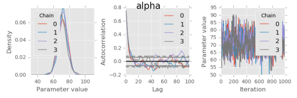
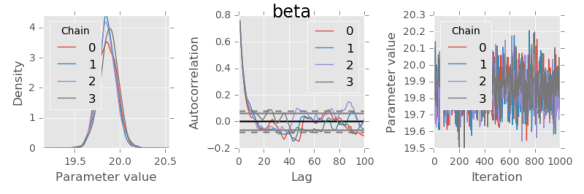
def plot(trace, var):
    fig, axes = plt.subplots(1, 3, figsize=(9, 3))
    fig.suptitle(var, fontsize='xx-large')

    # Marginal posterior density estimate:
    trace[var].plot.density(ax=axes[0])
    axes[0].set_xlabel('Parameter value')
    axes[0].locator_params(tight=True)

    # Autocorrelation for each chain:
    axes[1].set_xlim(0, 100)
    for chain in trace[var].columns:
        autocorrelation_plot(trace[var,:,chain], axes[1], label=chain)

    # Trace plot:
    axes[2].set_ylabel('Parameter value')
    trace[var].plot(ax=axes[2])

    # Save figure
    plt.tight_layout()
    fig.savefig('{}.png'.format(var))

# Display diagnostic plots
for var in trace:
    plot(trace, var)

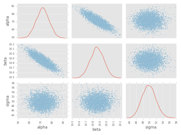
# Scatter matrix plot:
scatter_matrix(trace.to_frame(), diagonal='density')
plt.savefig('scatter_matrix.png')